RL Fundamentals and MDPs
In this post, we’ll try to get into the real nitty-gritties of RL and build on the intuition that we gained from the last article. So we’ll bring in some mathematical foundation and then introduce some RL parlance that we will use for the rest of this course. I’ll stick to the standard notation and jargon from the RL book.
Three Challenges
Before we begin with the mathematical foundations of RL, I’d like to point out three challenges in RL we need to account for if we were to come up with RL algorithms of our own. Once again, I’m going to move on to a new example so lets take chess this time.

So we want to teach our agent (recall what this means from the previous post) how to play the game of chess. Lets assume we have some sort of reward function in place where we get some small positive rewards for capturing a piece and small negative rewards for losing a piece depending on the importance of the piece (so losing a queen would lead to a negative reward of larger magnitude than losing a pawn). We also have some large positive final reward for winning the game and a large positive negative reward for losing. If you’re wondering whether just this large final reward is a sufficient reward function on its own, you’re probably right and it probably is, but lets stick to this for the sake of illustration.
Now assume we have an RL algorithm that can look at several games of chess and the rewards and learn to play chess on its own. What would this algorithm need to account for? We spoke about trial and error being the basis of any RL algorithm in the previous post that is exactly what our algorithm would do as well. It starts playing random moves and when it plays a good move (positive reward), it remembers to play that move the next time it is in a similar situation. This seems fine on the face of it, but there is an issue. Maybe the algorithm found a good move to play at a given position, but what if there was a better move?
We need some way for the algorithm to account for the possibility of there being a better move than the one it has found already. So when we train our agent we need to make sure the agent doesn’t greedily play the best move it knows all the time but also plays some different moves, hoping that they may be better than the one it already found. This is called the exploration-exploitation tradeoff in RL. Usually, RL algorithms tend to explore i.e. play many random moves initially and when the agent is more sure about the best moves under different circumstances, it starts exploiting that knowledge. We will revisit this problem in the next post with another example.
Lets move on to the next challenge that our RL algorithm will have to account for. Lets say our RL algorithm is learning from a game of chess again where the player sacrifices the queen but goes on to win the game. The RL agent immediately registers a negative reward for the loss of the queen but the large positive reward for winning the game only comes much later. But it is entirely possible that the very queen sacrifice that the RL agent probably classified as a bad move, was the reason for the player winning the game. So it is possible that a move seems like a “bad” one in the short term but in the long term, could be a very “good” move. How do we account for this in our algorithm? This is the concept of delayed rewards and we will deal with a simple yet elegant solution for this as well as we go through this post. We will look at another example for this as well in the next post.
And finally our RL algorithm should learn to generalize i.e. it should be able to efficiently learn from the data it collects. One of the major drawbacks in RL is that it requires a lot of data to learn so generalization is important for RL algorithms.
Note that RL is based on the reward hypothesis that states that:
All goals can be described by the maximisation of expected cumulative reward
Think about whether you agree with this statement.
With that background, lets talk about how RL problems are modeled and get into some math.
Markov Decision Processes
The future is independent of the past, given the present
Almost all RL problems can be modeled as a Markov Decision Process (MDP). So what is an MDP? An MDP is a mathematical model that we will be seeing a lot over this course. Most of our RL environments, will be MDPs. An MDP can be defined as a five tuple: $$\langle \mathcal{S}, \mathcal{A}, \mathcal{P}, \mathcal{R}, \gamma \rangle$$
Lets take a closer look at what all of this means. Note that in this section, I do not follow the notation in the RL book and follow the notation here which is quite commonly followed.
- S : This is the set of states of the MDP. In an RL setting, this would correspond to different settings of the environment i.e. each setting of the environment is a state in the MDP. In the previous post, we spoke about how RL was all about choosing the right actions at the right times i.e. depending on the state of the environment. This is the state we were talking about. A state in chess or tic-tac-toe could be the board positions or while riding a bike could be some combination of the pertinent variables like the angle of the bike with thr ground, the wind speed, etc. The S variable represents the set of all unique states in the MDP.
- A : This is the set of all actions of the MDP. We already spoke about actions briefly. Actions describe the possible moves in a game of chess or tic-tac-toe or different arrow keys or buttons in a video game, etc. It represents the different options the agent has and can play at a given point in time. A represents the set of all unique actions available to the agent.
It is worth mentioning that both S and A can be finite or infinite sets. Both can also be continuous spaces or discrete spaces, depending on the variables in the state space or the nature of actions. For example, if we have a variable taking real numbered values in the state space, the state space is automatically continuous (and infinite). If our actions are in the form of degree of turning a steering wheel, once again, continuous and infinite action space. A finite MDP has both finite S and finite A.
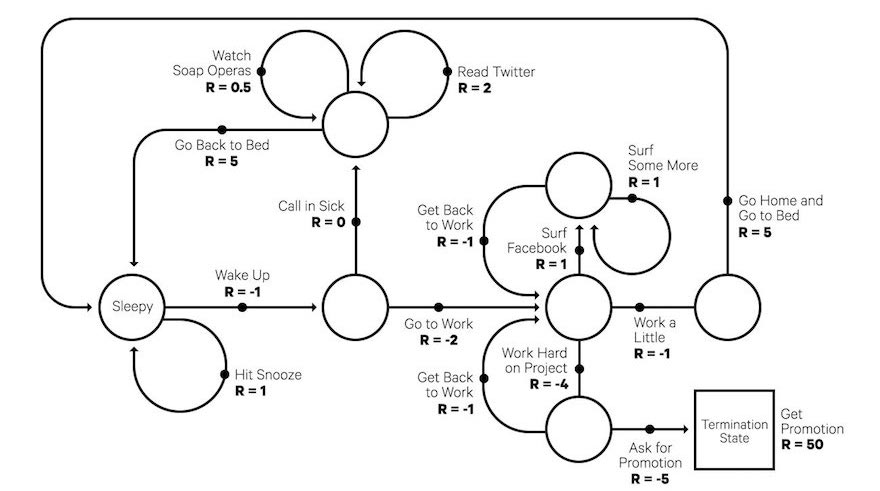
Before we move on to the other symbols, lets get some things clear. Here is another more detailed MDP for your reference.
Some of the states of the MDP are designated as start states or initial states and end states or terminal states. An episode in RL is a sequence of state-action pairs that take the agent from a start state to a terminal state. So the agent starts from one of the intial states, plays an action, goes to the next state and so on until it hits a terminal state and the episode ends. Assume for now that there is such an end i.e. every episode does end after some unknown, finite time. This is a property of finite horizon MDPs which is what we will stick to in this course.
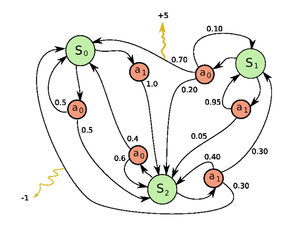
Now lets take a look at this MDP in the diagram above. Assume S0 is your initial state. Notice that a0 from S0 has two arrows, one going into S0 again and another going into S2. The numbers on the arrows indicate 0.5 and 0.5 respectively. This means that if an agent plays the action a0 from S0, it has a 0.5 probability that it ends up back in S0 and a 0.5 probability that it ends up in S2. And similarly we have arrows going all over the diagram. Also notice the wiggly arrows – they’re rewards.
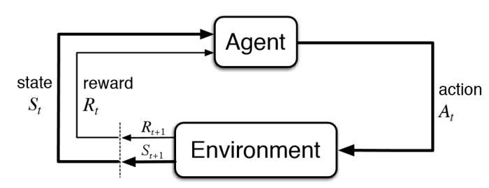
Notationally, we index the sequence of state-action pairs in an episode with a time variable t so we say an agent plays action at from state st and gets reward rt+1 for doing so (the reward can be 0). Here, t starts from 0 and we represent the terminal time-step as T.
Another crucial thing to note is that actions in an MDP have to be instantaneous in nature. That means you take action at from state st and end up in state st+1 immediately. There are several actions in real-world problems that may not be instantaneous but we’ll deal with them later. For now, assume your actions are instantaneous.
- P : Now P is the probability function defined as P(s'| s, a) which is read as the probability of moving to “state s'” from “state s” if the agent plays “action a”. So for example, P(S2|S0,a0) = 0.5. This is also called the transition function.
- R : This is the reward function or reinforcement function and is defined as R(s'| s, a) which is the reward the agent gets for moving to “state s'” from “state s” if the agent plays “action a”. So for example, R(S0|S1,a0) = +5. However, the answer may not be as simple as a single number and the reward could be sampled from a probability distribution i.e. R(s'| s, a) is a probability distribution that we will try to estimate by interaction with the environment. There are some other forms of reward functions like R(s,a) or even just R(s) as well. Note that rewards are always scalars because they are easier to optimize. They are also usually finite.
- $\gamma$ : We spoke about the concept of delayed rewards earlier in the post and we wanted a way to accound for delayed effects of actions. This is where $\gamma$ helps. We define the returns of an action from a given state as the sum of the discounted rewards we receive from that state for playing that action. If we started from the state s0, the returns would be defined as r1 + $\gamma$ r2 + $\gamma$2 r3 + … $\gamma$ T-1 rT. We use the word “discounted” because $\gamma$ is usually a number between 0 and 1 and with the increasing powers, we give more weight to the immediate rewards than the delayed rewards. Hence, $\gamma$ is also called the discounting factor. The symbol we use for returns from timestep t is usually Gt although some people like using R as well (r for reward and R for returns). We will stick to the former notation. Now going back to the queen sacrifice example, if we were to consider the returns in our algorithm instead of just the immediate reward, we will be able to account for the delayed positive effect and not just the immediate negative effect.
But with all of that information, we still haven’t covered that blockquote at the start of this section. No, that wasn’t a quote from Avengers: Endgame and it is the most important takeaway from this post. So what does it mean? Mathematically, it means this:
$$P(s_{t+1}|s_t,a) = P(s_{t+1}|s_t,s_{t-1},s_{t-2},s_{t-3},…,a)$$
But what does that mean intuitively? It means the probability of going to state st+1 from state st under the action a is independent of how we got to state st in the first place. If you’re thinking this isn’t very realistic, you’re right but this type of modeling works in most cases and is called The Markov Property. The future is independent of the past, given the present i.e. the action from the current state only depends on the current state and not how we got to this state in the first place.
We make another assumption of stationarity which means:
$$P(s_{t+1}=s',r_{t+1}=r|s_{t}=s,a_{t}=a) = P(s',r|s,a)$$
This means that the timestep variable doesn’t matter – no matter at what point we are in the trajectory, given the state s and and action a, we always end up sampling the next state s' and the reward r from the same distribution. This is a property of stationary MDPs.
And with that, we’ve covered MDPs and how to model RL problems. With this background, I also recommend reading this. But with that definition, we still haven’t accounted for the exploration-exploitation tradeoff. So in the next post, we’ll introduce a few more symbols and definitions before we get cracking with our very first RL algorithm!
Once again, let me know if you have any feedback or suggestions.