Policies, Value Functions and the Bellman Equation

In the last post, we discussed the three major challenges RL algorithms need to tackle and then went on to Markov Decision Processes (MDPs). We’ll start this post with a quick recap of some important concepts from the last post and then move on to new ideas.

An MDP formally describes the environment for RL when the environment is fully observable i.e. we know all the values of the relevant state variables. In other words, the current state completely characterises the process. Almost all RL problems are formulated as MDPs. This is the same MDP we saw in the previous post. We already discussed the different components of an MDP i.e. the states, the actions, the transition function, reward function and the discount factor $\gamma$. If you need to refresh your memory about any of these, refer back to the previous post before you go ahead. Here is the Markov property once again for your reference. The future is independent of the past given the present and the state captures all relevant information from the history. This means once we know what state we are in, we don’t care how we got to the state in the first place i.e. the state is a sufficient statistic of the future.

$$P(s_{t+1}|s_t,a) = P(s_{t+1}|s_t,s_{t-1},s_{t-2},s_{t-3},…,a)$$

More on Delayed Rewards

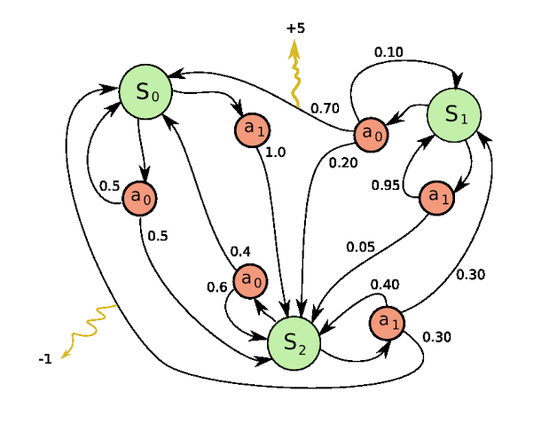
Lets quickly recap the idea of delayed rewards once again. Look at the MDP below (and please ignore all religious connotations that might be implied). Clearly in the MDP below, from earth, the right move is to go to Heaven since you get a reward of +1 in perpetuity even though you get a negative reward to make the transition in the first place. Although the transition to hell initially looks like a good move, you get a -1 in perpetuity and hence doesn’t work well in the long term.

Although this is not a finite horizon MDP (recall what this means from the last post), the idea is that we want to account not just for immediate gains but long term gains as well. We already saw how the discount factor and returns allow us to account for this. In fact a $\gamma$ close to 0 leads to “myopic” or “short-sighted” evaluation and a $\gamma$ close to 1 leads to “far-sighted” evaluation. We often pick a value in between 0 and 1 but closer to 1. We will revisit the returns definition later in this post.

More on the Explore-Exploit dilemma

Lets talk about the exploration-exploitation dilemma we referred to in the last post as well. Look at the figure given below.

The exploration vs exploitation dilemma exists in our everyday lives as well. Imagine your favorite restaurant is right around the corner and you’ve been there plenty of times. If you go there every day, you would be confident of what you’ll get, but you don’t know what you’re possibly missing. If you tried different places, you could occasionally be visiting a terrible place but you could also find a new place that is better than this one. So it makes sense to explore and try new places but once you have a good idea pf what’s in the area, you can start exploiting and go to your favourite place. This is exactly what we want our agents to do as well in RL. We want them to explore (randomly or based on some strategy) intially and when its sure of the best actions from each state, it can exploit that knowledge to gain high rewards.

More Jargon and Symbols

Now that we’re done with that recap, lets get on to some new material. This is the most important section of this post and perhaps the entire series so make sure you understand exactly what’s going on in this section.

Returns

We already discussed what returns are in the previous post, but here is the formal expression

$$G_t = r_{t+1}+\gamma r_{t+2}+…r_{T} = \sum_{k=t}^{T-1} \gamma^{k}r_{k+1}$$

We end the episode at the timestep T because we assume a finite horizon MDP. Remember that T is a random variable – for example when we play tic-tact-toe, the game could end in a different number of moves each time. Each of the independent $r_{k}$ terms are also random variables and hence, $G_{t}$ is also a random variable. Further, since each reward term is usually finite, the returns does not blow up to infinity. As we have already discussed, the discount factor is a number between 0 and 1 and often close to 1 and is chosen according to the problem at hand. Also recall that $r_{t+1}$ is the reward received by performing action $a_{t}$ at state $s_{t}$ ; $r_{t+1} = R(s_{t}, a_{t})$ where R is the reward function. So this means that $G_{t}$ is the returns accumulated from the state $s_{t}$. When we try to come up with RL algorithms we want to try and optimise $G_{t}$ at all points in the trajectory.

Policy

$$\pi_t(a|s) = P(a_t=a|s_t=s)$$

The policy is a mapping from states to actions or action distributions. The above eqation reads as the probability of taking an action a at time t given that the state at time t was s. A stationary policy is time-independent which means we can omit the timestep variable t. No matter at what point we are in the trajectory, under the policy, if we are at state s, then the action we take (or the probability distribution over the actions we can take) is the same. So unless we are specifically talking about non-stationary policies, we omit the t notation. Another important distinction is between stochastic and deterministic policies. A deterministic policy is a mapping $\pi: S \rightarrow A$ which is essentially a function that maps each state to a single action. A stochastic policy on the other hand maps each state to a probability distribution over all the actions. So a deterministic policy can be thought of as a stochstic policy where only the probability of one of the actions is non-zero.
In all RL problems, we want to learn the policy of the problem and we do this by either trying to learn the policy directly or by learning the policy through the following functions.

Value function

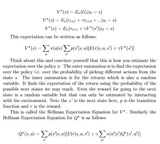
$$V^{\pi}(s) = E_{\pi}(G_{t}|s_{t}=s)$$

V is the value function of the state associated with the policy $\pi$. It is the expectation of the returns from the state with respect to the policy $\pi$. Note that $G_{t}$ itself depends on $\pi$ as the next reward depends on $\pi$. Since the V function is the expectation of the returns from the state, it tells us how good a state is i.e. what is the expected sum of rewards we can accumulate from a given state under the current policy. So it is a measure of “goodness” of a state.

Q function

$$Q^{\pi}(s,a) = E_{\pi}(G_{t}|s_{t}=s, a_{t}=a)$$

This is the Q-function and it is almost the same as the value function, except that here, the first action you take from state s is always a and then you follow the policy $\pi$ from then on. Like the value function, the Q-function tells us not only how good a state is but also how good it is to pick each action from the state. So if $Q^{\pi}(s,a1)$ is greater than $Q^{\pi}(s,a2)$ then it is better to choose action a1 versus action a2 in state s under the given policy. So it tells us the “goodness” of each action in the state. The value function and the Q-function are crucial for several RL algorithms that we will be seeing over the next few posts.

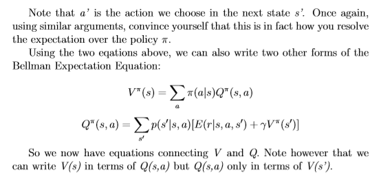
The Bellman Equation

If we were able to find the optimal value function of each state in the MDP or the Q-function of each state-action pair, then we have solved the RL problem. We will define what “optimal” means in the next section but for now, just understand that it means “the best in terms of collecting maximum rewards”. Because at each state, we keep moving to the next potential state with the highest value function (or the state with the potential to collect maximum returns). Or in terms of Q-functions, from each state, we play the action with the highest Q-function value from that state. So we’re being greedy with our choices and eventually we keep moving across states in the MDP in this manner until the episode ends. Since we move across states with the highest value function, we collect maximum returns along the way (by virtue of the definition of value functions and a similar argument is true for Q-functions).

But by doing this, we’re also learning a mapping from states to actions i.e. a policy. So if we have the estimates of the optimal value functions, we can estimate the optimal policy. This can be tricky to understand because we estimate the value functions using a policy and then we extract a policy by being greedy over the value function. But more on this later.

So if our estimates of the value functions and Q-functions are optimal, we will be gaining the maximum possible reward in the MDP and would have solved the RL problem. But how do we find the optimal Q-function values or value function values? Remember Q and V aren’t necessarily the optimal values, they are just the values under some policy $\pi$ (which may not be the optimal policy).

All of this probably seems confusing now but will be much clearer with the math in the images below and in the next section when we introduce some more simple equations. For now, it is important to understand the importance of trying to learn these “optimal” value functions and Q-functions.

Note that the Bellman Expectation Equations form a system of equations – one equation for every state. There are as many equations as there are number of states. The variables are $V^{\pi}(s)$ for all s. So we have n equations for n states and this system of equations will always have a unique solution because the transition matrix is a stochastic matrix. The equations are linear and they are solvable.

Optimality Equations

The aim of RL is to learn an optimal policy i.e. an optimal mapping from states to actions that can allow the agent to accumulate maximum rewards as it goes on a trajectory (governed by this policy) through the MDP. We want a $\pi$ such that for no other $\pi$ can we get better expected returns.

$\pi^{*} = \underset{\pi}{\operatorname{argmax}} E_{\pi}[G_{t}|s_{t}=s] \forall s$

And this can be written as:

$\pi^{*} = \underset{\pi}{\operatorname{argmax}} V^{\pi}(s) \forall s$

Here, $\pi^{*}$ is the optimal policy. The $\forall s$ tells us that this is true at any starting state or even any state in the trajectory. Note that there may be more than one optimal policy and in that case, we will take any one of them. However, even though there are several possible optimal policies, there is only one possible setting for the optimal value functions, i.e. there may be several optimal $\pi^{*}$ but there can be only one optimal $V^{\pi^{*}}$. Think about this for a second and convince yourself that this is in fact true.

$V^{\pi^{*}} = \underset{\pi}{\operatorname{argmax}} V^{\pi}(s) \forall s = V^{*}$

$V^{*}$ is the optimal value function. The existence of such an optimal value function and hence an optimal policy that is able to reach the maximum value function for all states has been proven in finite MDPs (it gets trickier in infinite MDPs but still holds for some settings). The proof is quite intricate but I have attached some notes from this NPTEL course in the reference section for the interested reader.

The math in the following images talk about the Bellman Optimality Equations. Once again, this is very important for the rest of the course.

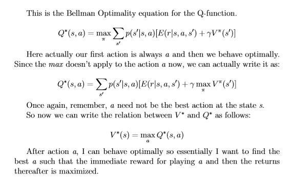
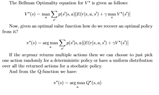
Now if we could solve the Bellman Optimality Equations, we would be done but unfortunately because of the max operator, the equations are non-linear and cannot be solved easily. So we need to think about how we can solve this problem.

Phew! That was a long post with a lot of information to take in but it is extremely important that you understand the ideas in this post clearly. In the next post, we’ll move on to our first RL algorithm so make sure you check it out!

Let me know if you have any feedback or suggestions.

References

1. Proof of the existence of an optimal value function in finite MDPs