Inverse Reinforcement Learning

This is a review of the paper Algorithms for Inverse Reinforcement Learning. I recommend some reinforcement learning (RL) basics before you read this. The first couple of posts from the RL course on my page might be a good starting point.

Inverse RL (IRL) is a topic I’ve been interested in in recent times so I’m excited to write this post. So lets get cracking!

The Problem

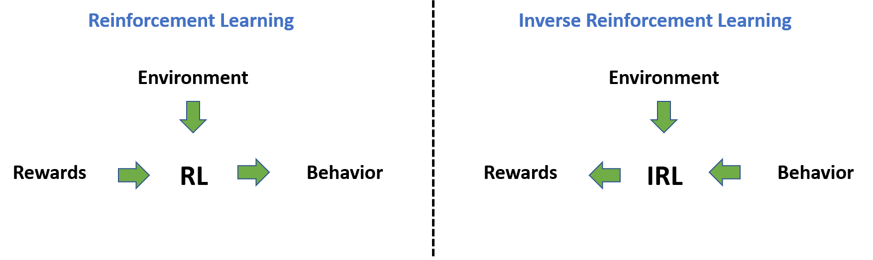
Reinforcement Learning has allowed researchers to solve several challenging problems without direct supervision but with some sort of distant/ weak supervision or feedback signal. In RL, this feedback signal is in the form of a reward signal. Reward functions are crucial to developing powerful RL models but coming up with good reward functions can be a challenging task. If we were to taake a game like Tic Tac Toe, the reward signal just presents itself based on the result of the game. If it were a video game we were trying to learn, then once again the score in the game provides a solid reward signal. But what about in the case of self-driving cars? With so many factors to consider, it is difficult to come up with a good reward function and even if we do, there may be a better reward function possible. Researchers recognized this issue with RL and decided to come up with a way to learn a reward function. They wanted to learn a reward function from optimal behaviour. So they would look at a human driving a car, learn a reward function from the demonstration, and then use this reward function to train an RL agent. The problem of extracting the reward fnction from observed optimal behaviour is the problem of Inverse Reinforcement Learning (IRL).

Inverse Reinforcement Learning: Find a reward function to explain observed optimal behaviour

The paper gives two major motivations to learn such a reward function. One is obvious: to use the reward function to train RL agents. Two, is to use with apprenticeship learning or imitation learning to teach agents.

The reward function and not the policy is the most succinct, robust and transferable definition of a task

Some Quick Pointers

Before we get into the meat of the paper, here are some quick pointers to keep in mind.

• All reward functions are only functions of the state and not the state and the action. So we have R(s) and not R(s,a) everywhere. This is done to simplify the math and the extension is simple. It may help to think of R as a vector of size N where N is the number of states.
• All values of the reward vector are bounded by a magnitude of Rmax
• Pa is a NxN matrix where Pij is the probability of going from state i to state j by playing action a.
• The paper uses the MDP setup for its proofs and arguments. Here are some properties and theorems that they take advantage of.

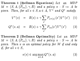
IRL in finite state spaces

So we need to find a reward function that explains our optimal behaviour. In this case, let us assume we have a finite state space of size N. The paper proves the following theorem using the properties above. The proof is quite simple to follow so I won’t talk about it here.

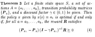
Now what does this theorem tell us? This theorem has now characterized our solution set. We’re no longer looking for a needle in a haystack. Initially, our reward vector R could have been any real vector of size N. But now, we have some constraints. R has to satisfy the above condition.

But the authors point out two issues.

1. R=0 is always a solution. If the reward function is the zero vector, then any policy is an optimal policy and so is our observed policy. The authors point out that this can be alleviated by demanding that our observed policy be the only optimal policy but this doesn’t work entirely because although we can get rid of the zero vector now, some vectors arbitrarily close to the zero vector would still be solutions.
2. We have characterised our solution set, but there are still several vectors that satisfy this condition. Which of those is our reward function?

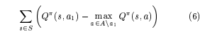
To address these issues the authors came up with a linear programming (LP) formulation to find the “best” R vector. The authors sought to maximize the sum of the difference between the quality of the optimal action and the next best action.

So maximizing the above should give you the reward function but the authors also claim that smaller rewards lead to simpler reward functions and hence want to control the magnitude of the R vector. To do this, they add a penalty term of $\lambda\Vert R\Vert_{1}$. $\lambda$ is a hyperparameter they control and larger the $\lambda$, the smaller the R vector norm and simpler the reward function. But this is a trade-off since you also want to maximize the first term. The authors claim that there is a phase transition point $\lambda_{o}$, such that if $\lambda > \lambda_{o}$, R=0 and if $\lambda < \lambda_{o}$, R is bounded away from 0. So the best $\lambda$ would be a value just below $\lambda_{o}$.

So the final optimization objective is as follows.

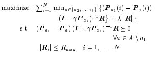
Note that the summation term running from 1 to N is so that we maximize across all the states in the MDP. Also note that we use our information of the optimal policy implicitly here since we know the best action a1 at every step. This can be solved as a LP problem now.

IRL in large state spaces using linear function approximation

We now consider a large (possibly infinite) state space. Assume we have n variables in our state space and so think of R now as a function $\Re^n \rightarrow \Re$.

But we don’t want to consider all such functions so let us restrict ourselves by only considering functions in the following format. We have used linear function approximation here.

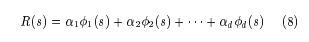
The \phi functions are basis functions over the state variables and our job now is to find the $\alpha$ values. Once again, since we’re using linear function approximation, we can use LP to solve the problem.

The paper also shows that the value function under a given policy is also a linear function of the $\alpha$ values (refer to the paper to see why this is true). So now, we can rewrite the equation that characterizes our solution set as the following for the large state space case.

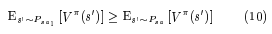
But we have a problem now. This leads to infinitely many constraints to check because the state space could be infinite and we need to check the condition for each one of those states. Remember we had a summation in the final equation in the last section? That would be an infinite summation in this case. However, the authors circumvent this issue algorithmically by just sampling a large number of states and just checking for those states.

The other issue is that since we have restricted ourselves by using linear function approximation, we may not be able to express all reward functions and hence we’ll relax some constraints and pay a penalty when we don’t meet the constraints. The final optimization objective is below.

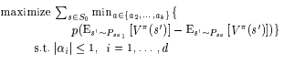
So is the subsample of states and $p(x) = x$ when $x \geq 0$ and $2x$ when $x < 0$. $\pi$ is the optimal policy. This can be solved with LP now.

IRL from sampled trajectories

Now, we come to the most interesting and most realistic case. We now try to learn from sampled trajectories from the environment. We do not require an explicit model of the MDP but we do assume the ability to find an optimal policy under any reward function. We also assume the ability to simulate trajectories in the environment with the optimal policy or any other policy we want. Also assume there is only a single start state so. This is not a string assumption as if there are several start states with an initial state distribution, add an additional state and connect it to each of them. This is the most realistic case and is different from the previous cases because we don’t have the model of the environment i.e. the P matrices.

Once again, R will be expressed as a linear function approximation in the same form as the previous section. Please refer to the paper and convince yourself that it is possible to use Monte Carlo trajectories to estimate a value function that is also linear in the $\alpha$ values. The math is quite simple and straight-forward. This is important because it allows us to use LP again.

So now we have the optimization objective as follows.

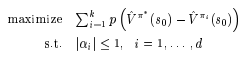
p is as defined in the previous section. But what is k in the summation? It is the number of policies apart from the optimal policy we are considering at that step of the algorithm. This will be clear in a second. The algorithm is as follows:

1. Start with the optimal policy $\pi^*$ and another random policy $\pi_{1}$. Find the $\alpha$ values that satisfy the above with k=1. Hence find R.
2. Now using the R we just found, find $\pi_{2}$ that maximizes $V^{\pi_{2}}(s_{o})$. This can be done using some RL algorithm.
3. Now add $\pi_{2}$ to our current set of policies and optimize the above for $\pi^*$, $\pi_{1}$ and $\pi_{2}$ with k=2.
4. Keep going until you are “satisfied”.

I will not get into the experiments conducted but I would highly recommend that you read the paper since there are some interesting details and observations.

Future Work

The authors plan on finding not just simple reward functions as they have done in this paper i.e. ones with small values but want to do one better to find “easy to learn” reward functions. I guess this means that “simple” doesn’t always mean “easy to learn”. They also want a way to be able to account for variation and noise in the state space and action selection process in real world applications. They also hope to find “locally consistent” reward functions in specific regions of the state space if they find that observed behaviour is far from optimal.